


Introduction
Materials and Methods
Data
Model specification
Results and Discussion
Preliminary tests and lag selection
Granger causality test results
VARX model estimation results
Impulse response and FEVD results
Implications and policy considerations
Conclusion
Introduction
Per capita egg consumption in 1980 was 119 eggs, rising to 348 eggs in 2021, a 192.44% increase over 41 years (MAFRA, 2025). Recently, however, growth in egg consumption has begun to slow, and fourth-quarter 2025 egg sales volume decreased by 3.1% year-on-year due to price increases. This suggests that egg consumption decreased after the Chuseok peak season as selling prices increased (Noh and An, 2026).
The decrease in egg consumption does not simply reflect a change in consumers’ purchase preferences; it is also an important signal of how price increases are reflected in the final stage of consumption. Eggs are a protein-rich food and are widely consumed due to their low cost (Zhang and Ji, 2024). Therefore, given that eggs are a representative basic food and a low-cost source of protein, a sharp increase in retail prices is highly likely to directly increase consumers’ purchase burden and reduce consumption. From the producer side, price increases do not necessarily translate into stable income gains because the extent to which retail price changes are passed through to farm-level prices may vary with the distribution structure. Therefore, the recent decrease in egg consumption and the increase in prices call for an analysis of the price transmission structure by distribution stage in the egg market.
Egg distribution is broadly divided into the farm-level stage (the production site), the wholesale stage (intermediate distribution), and the retail stage (final consumption). In terms of the distribution flow, farm-level price increases are passed on to the wholesale stage, and that higher price is then passed on to consumers. However, in the actual egg market, it is frequently observed that changes in farm-level prices are not smoothly transmitted to wholesale and retail prices, or that the transmission is delayed. In such cases, incomplete or delayed price transmission may lead to inefficiencies in resource allocation. Consumers may not fully benefit from price declines at upstream stages.
Incomplete or delayed price transmission across distribution stages may be associated with market frictions, such as information asymmetry among distribution actors, the market power of specific market participants, and menu costs (Hwang and Park, 2013). When information asymmetry exists, market participants at one distribution stage may be unable to fully observe changes in actual prices or supply and demand conditions at other stages (Aker, 2010). This may delay the transmission of price signals and the resulting adjustments in transactions and prices, leading to incomplete or delayed price transmission. When market participants at a particular distribution stage have pricing power, they may pass price increases from upstream stages on to downstream prices more quickly than price decreases to maintain their margins (Peltzman, 2000). Due to menu costs associated with repricing, retail prices may not be adjusted immediately even when upstream prices change (Mankiw, 1985). Inventory management, contractual arrangements, and promotional strategies may also delay short-run retail price adjustments. When incomplete or delayed price transmission is accompanied by price rigidity, a considerable amount of time may be required to resolve excess supply or excess demand caused by external shocks and to return prices to equilibrium (Seo and Shin, 2014).
To date, various studies have been conducted domestically and internationally on the causal relationships and price transmission in livestock products (Goodwin and Holt, 1999; Lee and Yoon, 2016; Joo and Lim, 2021; Bareith et al., 2025). Since few studies have directly analyzed price transmission in the egg market, research on livestock product markets provides an important basis for understanding the price transmission structure of eggs. Analyses have been conducted on the causal relationships and price transmission of livestock products using generalized autoregressive conditional heteroskedasticity (GARCH), autoregressive distributed lag (ARDL), error-correction model (ECM), and vector autoregression (VAR) models (Cha and Kim, 2009; Kim and Kim, 2009; Jeong and Huh, 2000; Kim and Nam, 2015; Joo and Lim, 2021). While some studies have analyzed the price transmission of eggs (Kang, 2011; Lim and Cho, 2012; Hwang and Park, 2013; Mun et al., 2020), they mainly conduct long-term trend analysis using monthly data. Few studies have analyzed the dynamic price transmission structure among farm-level, wholesale, and retail egg prices using daily data.
Meanwhile, including relevant external factors as exogenous variables allows their effects to be accounted for, thereby enabling the dynamic relationships among price variables to be estimated more appropriately. In livestock product markets, external factors can significantly influence supply, demand, and price conditions (Lee et al., 2021; Kim et al., 2022). Supply shocks caused by natural disasters, weather, disease outbreaks, and other factors may affect livestock product prices, including egg prices, and demand shocks arising from events such as population growth, industrial expansion, holidays, or panic buying may likewise affect the market (Tomycho et al., 2023). Previous studies have shown that highly pathogenic avian influenza (AI), movement restrictions, temperature, and short-term increases in demand can affect price formation or price transmission in livestock product markets (Zamani et al., 2022; Tomycho et al., 2023; Ajoseh et al., 2025; Pinem et al., 2026). However, there is little research on the effects of external shocks on the daily price transmission structure of eggs.
This paper analyzes price transmission in the egg market by distribution stage through a vector autoregression with exogenous variables (VARX) using daily data and considering external shocks. These external factors may operate through different primary pathways: distribution constraints for AI-related movement restrictions, farm-level production for heat waves, and demand and shipment timing for holidays, while all factors were jointly incorporated into the equations for all distribution stages. This study examines how price changes in one distribution stage are transmitted to other stages, how farm-level, wholesale, and retail prices respond dynamically to shocks, and how external factors affect price movements in each distribution stage. This study aims to identify the dynamic price transmission structure of the egg market and determine whether price transmission to the retail stage is delayed.
Materials and Methods
Data
Farm-level, wholesale, and retail egg prices were obtained from the Korea Institute for Animal Products Quality Evaluation. Only extra-large (XL) eggs were used due to data availability. Farm-level and wholesale prices are available for both 10-egg and 30-egg packages during the analysis period (January 1, 2020 - December 31, 2025); however, the 10-egg retail price is available from January 1, 2022 onward. Therefore, to reflect as much of the analysis period as possible, 30-egg package data with daily data were used. The days when the market was open were arranged chronologically and analyzed; days when the market was closed were excluded. The descriptive statistics for the egg price variables and external factors are shown in Table 1. Over the analysis period, 1,479 observations were recorded, with daily average egg prices of 4,786 won (farm), 5,163 won (wholesale), and 6,630 won (retail). The price change rate was calculated by first differencing the log prices. Accordingly, the number of observations for the price change rate decreased by 1 to 1,478, and the mean was 0.000 across all stages. The daily standard deviation was found to be at the level of 1.3 - 2%.
Table 1.
Descriptive statistics of egg price variables and external factors.
In this study, external supply factors were defined as movement restrictions due to AI and heat waves. When highly pathogenic AI occurs, culling or preventive culling is implemented for the affected farm and nearby farms. Eggs, chicks, and adult chickens are all culled during culling or preventive culling. Since it takes approximately 17 - 24 weeks for chicks to become adult chickens after they are born, it takes a considerable amount of time for the corresponding farm to supply eggs. Thus, when AI occurs, it affects the market for some time, even after the outbreak. However, because few studies use daily data, there is no clear standard for the number of days in the affected period following an AI outbreak. Setting the effect period to 3 days, 1 week, or 2 weeks based on the date of AI occurrence and encoding as a dummy variable may introduce arbitrariness in establishing the effect period.
Meanwhile, AI is highly contagious. In severe cases, movement restrictions are implemented for all poultry farms nationwide. When movement restrictions are implemented, access to laying hen and egg farms is limited, and supply-side constraints impede the flow of supply from the farm to the wholesale stage. Therefore, rather than using the date of disease occurrence, this study adopts the implementation of movement restrictions as the AI variable, as it better reflects the actual distribution constraint. Lastly, during heat waves, supply disruptions may result from reduced egg production in chickens and increased mortality among them. Holidays were identified as an external factor affecting market conditions, as demand for holiday foods, including those containing eggs, peaks 2 weeks before the holidays. This study incorporated these external factors and constructed the VARX model.
The AI effect refers to movement restrictions due to AI. The AI effect variable was constructed using official movement-restriction data for the period 2020 - 2025 announced by the Ministry of Agriculture, Food, and Rural Affairs. If movement restrictions occurred in at least one place nationwide for laying hens, chickens, or poultry, it was set to 1; otherwise, it was set to 0. Heat wave data were obtained from the Open MET Data Portal of the Korea Meteorological Administration, where heat wave days are defined as days on which the daily maximum temperature is 33℃ or higher. It was assigned a value of 1 if there was a heat wave in at least one region nationwide, and 0 otherwise. Holidays were set to 1 from 2 weeks before the holiday date to the day before the holiday, and 0 otherwise.
Model specification
This study used a VARX model to analyze the price transmission structure by egg distribution stage. By incorporating factors external to the price system as exogenous variables, the VARX model allows external influences on price dynamics to be explicitly accounted for (Nicholson et al., 2017). Moreover, as a multivariate time-series model, it enables price change rates at different distribution stages and their dynamic interrelationships to be analyzed jointly rather than separately (Tsay, 2005). The VAR model estimates the stochastic process of a time series using linear regression equations, in which the current observed values of related variables are treated as dependent variables (Lütkepohl, 2006). Past observed values of these endogenous variables are used as explanatory variables, and exogenous variables are incorporated into the VARX model (Ocampo and Rodríguez, 2012).
As the endogenous variables of this model, the farm-level , wholesale , and retail price change rates were set, and the multivariate time series vector was defined as follows:
To ensure consistent units of analysis and to consistently identify the dynamic process of price transmission, all log prices were first-differenced and applied to the model. In addition, to control for external factors in the egg market, the AI effect, heat waves, and holidays were included as the exogenous variable vector . Drawing on this, the VARX model with lag can be expressed as follows:
where is the (3 × 3) coefficient matrix for the lagged values of the endogenous variables, 𝛤 is the coefficient matrix for the exogenous variables, is the lag order, and is an error term that follows a normal distribution with a mean of 0 and variance–covariance matrix 𝛴. The error terms of each variable have contemporaneous correlations with each other. The error term can be decomposed into a linear combination of structural shocks , which are mutually independent. If the relationship between the two error terms is a matrix, it is expressed as follows:
where , , and denote the unique price shocks of the farm-level, wholesale, and retail markets, respectively, and are assumed to be mutually orthogonal. The relationship holds. The variance–covariance matrix 𝛬 of the structural shocks has the form of a diagonal matrix in which all off-diagonal elements are 0, as follows:
The recursive structure means that shocks to the farm-level price, the upper stage, have an immediate effect in the current period on the wholesale and retail prices, the lower stages. However, the unique shock at the retail stage is not immediately transmitted to the upper stage.
To identify structural shocks, Eq. (2) was estimated using ordinary least squares, and the variance–covariance matrix of the residuals, , was derived. Then, this was Cholesky-decomposed, and the matrices and 𝛬 were estimated as follows:
Once the VARX model is identified, to obtain the spillover effects of a shock to a specific variable on other variables, the endogenous innovation process of the VARX model can be transformed into a vector moving average conditional on the exogenous variables as follows:
If the above equation is reconstructed as a function of mutually orthogonalized structural shocks , the following impulse response function can be obtained:
where the elements of the matrix represent the degree to which a one-unit structural shock that occurs in market at time affects the price of another market after periods (). In the impulse response, if the value approaches 0 as s increases, the effect of the shock is temporary; otherwise, it is permanent (Park and An, 2009).
Finally, forecast error variance decomposition (FEVD) can be performed to obtain the relative contribution of each structural shock to the forecast error variance of the endogenous variables. The contribution of the forecast error variance of the structural shock in market to the price volatility in market after periods is calculated as follows:
where denotes the contribution of the -th structural shock to the forecast error variance of the -th variable after periods, and m denotes each structural shock of the three endogenous variables.
Results and Discussion
Preliminary tests and lag selection
As shown in Table 2, the augmented Dickey–Fuller (ADF) unit root test, performed to assess stationarity by egg distribution stage, indicates that the log prices at the farm and wholesale stages were nonstationary at the 5% significance level. However, the log price of the retail stage was found to be stationary in levels. Retail prices rejected the unit root null hypothesis at the 1% significance level, and wholesale prices rejected it at the 10% significance level, both supporting stationarity. At the 5% significance level, the p-values for farm and wholesale prices were 0.421 and 0.097, respectively; unlike retail, they did not support stationarity. When the null hypothesis is that a unit root exists, low test power may prevent rejection even when the time series is stationary. To ensure stationarity, the log prices were first-differenced, and the ADF unit root test was additionally performed on the price change rates. As a result, in all distribution stages, the null hypothesis that a unit root exists was rejected at the 1% significance level. Accordingly, it was confirmed that stationarity was supported in the price change rates of all distribution stages.
Table 2.
ADF unit root test results for egg price variables.
| Distribution stage | Original price | Log price | Price change rate |
| Farm-level | -1.603 | -1.721 | -49.593*** |
| Wholesale | -2.473 | -2.580* | -56.859*** |
| Retail | -6.967*** | -6.975*** | -38.305*** |
Table 3 presents the lag-criteria comparison results for the VARX model. Selecting the appropriate lag is important when using the VARX model. If the lag is set to a long value, the autocorrelation of the residual term decreases, but inefficiencies may occur. To address this, after constructing an unrestricted VARX model using data for which the time series has been tested for stability, the appropriate lag should be selected. Based on the final prediction error (FPE) and Akaike information criterion (AIC), lag 12 minimizes both criteria, while the Hannan–Quinn information criterion (HQIC) and Schwarz Bayesian information criterion (SBIC) criteria select lags 8 and 4, respectively. This study focuses on short-run price dynamics using daily data; thus, the FPE and AIC criteria were prioritized to retain sufficient lag information and reduce the risk of omitting relevant adjustment dynamics. In general, the effects of shocks tend to be transmitted across distribution stages with a lag rather than being reflected immediately because of information transmission and inventory adjustment processes. Given the daily data, a lag of 12 was considered sufficiently long to capture potential lagged responses to shocks across the distribution stages. Therefore, this analysis was performed using the VARX model with a lag of 12.
Table 3.
Lag criteria comparison results of the VARX model.
Table 4 shows the results of the Johansen cointegration test. If a cointegration relationship is established, a long-term equilibrium relationship can be considered in the analysis. As a result of the previous ADF unit root test at the 5% level, the farm-level and wholesale log prices were nonstationary time series. However, since this study aims to identify the dynamic relationship within a multivariate system rather than a single variable, the Johansen (1991) cointegration test was performed using a lag of 12 (Table 3). The test shows that the trace statistic rejected all null hypotheses at the 5% significance level, and the system had full rank equal to the number of variables. For multivariate time-series analysis, when external factors are included as exogenous variables, a vector error correction model (VECM) or VARX model may be considered depending on the stationarity and cointegration structure of the endogenous variables. In general, a full-rank result indicates stationarity of the level system in the Johansen framework, whereas a conventional VECM requires a reduced-rank cointegrating structure. Therefore, a conventional VECM was not applied; instead, the analysis was conducted using a VARX model. Based on the ADF test results, the model was estimated using price change rate data derived from first differencing the log prices.
Table 4.
Johansen cointegration test results.
| Variables | Optimal lag | Cointegration rank | Trace statistic | 5% critical value |
|
Farm-level, wholesale, and retail log prices | 12 | r = 0 | 68.82** | 29.68 |
| r ≤ 1 | 29.78** | 15.41 | ||
| r ≤ 2 | 8.23** | 3.76 |
Granger causality test results
After determining the lag, the hierarchical order of the variables should be determined. The residuals from the VARX model are correlated. To analyze the dynamic relationships among variables for errors that are orthogonal and uncorrelated, impulse response and variance decomposition analyses will be conducted later. To obtain orthogonalized errors, the variance–covariance matrix is computed from the residuals, and then the errors are obtained via Cholesky decomposition. Since the structure varies with the hierarchical order of the variables, it affects impulse response analysis and variance decomposition analysis (Ocampo and Rodríguez, 2012).
The results of the Granger causality test to determine the hierarchical order of price change rates by distribution stage are shown in Table 5. The Granger causality test derives a predictive causal relationship, or Granger causal relationship, for a functional relationship when the causal relationship among variables is not transparent in regression analysis. The Granger causality test at lag 12 reveals that the farm-level price change rate Granger-causes the wholesale price change rate at the 1% significance level, but not the retail price change rate. The wholesale price change rate also Granger-causes the farm-level price change rate at the 1% significance level, but not the retail price change rate. The retail price change rate does not Granger-cause either the farm-level or wholesale price change rate. That is, the change rates of the farm-level and wholesale prices Granger-cause each other at the 1% significance level, whereas the remaining relationships were not statistically significant. This pattern suggests that predictive linkages are concentrated between the farm-level and wholesale stages rather than extending to the retail stage.
Table 5.
Granger causality test results.
VARX model estimation results
The results of the VARX model are shown in Table 6. The VARX model was estimated with a lag of 12, as determined above, and variables were ordered according to the distribution stages: the change rates of farm-level, wholesale, and retail prices. The analysis shows that the change rates of the farm-level and wholesale prices were statistically significant at the 1% level for their change rates one period before (). However, the change rate of the retail price had little effect on its own price change rate one period before.
Table 6.
Estimation results of the VARX model.
The effects of price change rates 12 periods earlier on each price change rate were examined. Farm-level price change rates were statistically significant in explaining their own dynamics (at the 5% level) and wholesale price change rates (at the 10% level), yet retail price change rates were not statistically significant at any distribution stage at the 12th lag. The external factors were also analyzed in the VARX model. The AI effect was statistically significant at the 10% level for the retail price change rate, and the holiday factor was statistically significant at the 1% level for the farm-level price change rate and at the 5% level for the retail price change rate. The heat wave factor was not statistically significant. Although heat waves are generally closely associated with livestock production, this result may reflect the construction of the nationwide dummy variable, which does not capture variation in heat exposure across egg-producing areas.
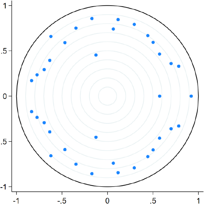
If the VARX model’s system is unstable, the effect of shocks may not converge, and the impulse response analysis and FEVD analysis to be conducted later may yield unreliable results. Therefore, it is first necessary to test the stability of the VARX model. In the stability test of the VARX model, if all observations plotted as points lie within the unit circle and the roots are smaller than 1, the model is considered stable (Kim and Nam, 2015). As shown in Fig. 1, all points corresponding to observations of price change rates of eggs by distribution stage lie within the unit circle; thus, the VARX model is stable.
Impulse response and FEVD results
Although the VARX model explains short-term effects well, its estimates do not directly show how shocks propagate over time. To address this limitation, the study performs impulse response analysis and FEVD analysis to analyze how the mutual effects influence their own and other variables over time (Kim and Nam, 2015). Table 7 shows the results of the impulse response analysis for price change rates, and Figs. 2, 3, 4 show the same results for each distribution stage. Given that the endogenous variables are price change rates derived from first-differencing the log prices, the impulse response values do not represent direct changes in price levels.
Table 7 and Figs. 2, 3, 4 show that shocks to the error terms of the change rates of egg prices at each distribution stage have effects over 15 periods, corresponding to lag 15 (about 3 weeks later). When a one-unit shock was applied to the error terms of the price change rates by all distribution stages, the spillover effects of the shock rise and fall, with most converging to 0 after about 15 periods.
As a result of the impulse response analysis, a one-unit shock to the farm-level price causes the farm-level price itself to respond most strongly, and the wholesale price also shows a relatively clear response. By contrast, the retail price response was found to be insignificant. When a one-unit shock occurs in the wholesale price, the wholesale price itself responds most strongly, and the farm-level price shows a relatively clear response, while the response of the retail price is statistically insignificant. Lastly, a one-unit shock to the retail price causes the retail price itself to respond most strongly, while the responses of the farm-level and wholesale price change rates were generally small. This indicates that price shocks in the retail market had limited effects on the farm-level or wholesale markets.
Like the Granger causality test, the results of the impulse response analysis show that the farm-level and wholesale price change rates in response to each other’s price change rates were larger when excluding their own price change rates. The retail price change rate generally showed an insignificant response to the farm-level and wholesale price shocks. This may reflect price rigidity, in which shocks from higher stages of the distribution are not immediately reflected at the retail stage. Since the shocks to the error terms of the egg price change rates by distribution stage mostly converged to 0 after about 15 periods, it was considered that policies to mitigate these shocks may be more effective if implemented quickly within this period.
Table 7.
Impulse response results for price change rates.


FEVD analysis is effective at identifying the relative importance of individual variables affecting the model, such as farm-level, wholesale, and retail price change rates (Kim and Nam, 2015). How much of the forecast error variance of the egg price change rate by each distribution stage is explained by the individual variable itself, and other variables in the current period and past lags was examined using FEVD analysis over approximately three weeks. Table 8 presents the FEVD results for the price change rates, and Figs. 5, 6, 7 show the same results for each distribution stage.
According to the FEVD, the farm-level price change rate was mostly explained by its own factor. After 1 period, the portion explained by the change rate of the farm-level price itself was 100.00%; after 12 periods, it was 96.81%, indicating that most of the variation could be explained by the change rate of its own price. However, as the lag increased, the share attributed to its own factor slightly decreased. In contrast, the effect of the wholesale price, which is at the lower end of the distribution, increased, indicating some backward transmission.
In the case of the wholesale price change rate, after 1 period, the portion explained by the change rate of the farm-level price was about 7.55%, whereas the part explained by the change rate of the wholesale price itself was about 92.45%. However, after 12 periods, the share explained by the wholesale price change rate decreased to 88.93%, while the share explained by the farm-level price change rate slightly increased to 10.31%. This shows that the wholesale price change rate is mainly explained by its own price change rate, but the effect of the farm-level price also increases over time.
For the retail price change, after 1 period, about 0.06% was explained by the farm-level price change, 0.01% by the wholesale price change, and 99.93% by the retail price change. This effect persisted, reaching 99.17% after 12 periods. This result indicates weak price transmission from the upper distribution stages to the retail stage and is consistent with potential retail price rigidity.
In summary, at the farm level, as the forecast horizon increased, some backward transmission was observed. In contrast, at the wholesale stage, some forward transmission occurred. The retail price change rate has a relatively independent structure, showing weak short-run connections with farm-level and wholesale price changes, which may reflect price rigidity.
Table 8.
Forecast error variance decomposition results.


Implications and policy considerations
In terms of implications, there may be scope for differentiated policy responses by distribution stage. At the farm level, shipment coordination, producer price stabilization, and pre-holiday supply planning can be considered. The VARX analysis indicated significant negative effects of the holiday factor on farm-level and retail price change rates. The decline in retail prices may temporarily reduce the price burden on consumers during the holiday period, whereas the decline in farm-level prices may reflect increased supply to meet peak holiday demand. Therefore, timely price information and shipment coordination may facilitate price adjustment at the farm level. Producer protection policies may also be considered to address periodic declines in farm-level prices, including measures that encourage farms to distribute shipments before and after holidays and protect the farm-gate prices received by producers.
At the wholesale stage, logistics resilience and inventory management may be considered. Although the AI-related movement restriction variable was statistically significant only at the retail stage, movement restrictions may disrupt the flow of physical supply through the wholesale and retail stages. Distribution infrastructure may therefore need to be strengthened to respond to livestock disease shocks. In particular, the supply chain response system at the wholesale stage could be reinforced to support a more stable supply to the retail market. Even when strict movement restrictions are implemented, supply chain resilience could be enhanced by flexibly adjusting the frequency and quantity of deliveries from wholesale hubs to retail markets.
At the retail stage, improvements in price adjustment mechanisms could be encouraged, and greater transparency in the distribution network could be considered. The FEVD analysis shows that, even after 15 periods, the retail price change rate’s own shocks accounted for a high proportion of its forecast error variance, indicating weak connections with the farm-level and wholesale stages. This suggests that price changes at the upper distribution stages are not fully transmitted to the retail stage. However, weak price transmission may arise not only from retail price rigidity but also from retail pricing strategies, menu costs, contractual arrangements, or inventory behavior. To improve price adjustment and transparency, strengthening the collection and distribution system centered on egg distribution centers may be considered, and price information by distribution stage could be disclosed more systematically. The monitoring and disclosure of retail margins and distribution costs can also be considered to improve transparency in retail price formation. In addition, auctions at public wholesale markets and online direct-transaction platforms may help facilitate smoother price adjustments among distribution actors.
It is also necessary to strengthen agricultural observation and early-warning capacity using high-frequency daily data. The current supply and demand policy mainly relies on monthly or quarterly observation data and, therefore, has limited ability to respond preemptively to rapid market changes. Therefore, the agricultural observation system could be enhanced to monitor egg distribution prices daily by integrating it with big data and point-of-sale data. To this end, establishing a real-time early-warning system may be considered to prepare for instability in egg supply and demand.
Conclusion
This study examined the causal relationship and price transmission by distribution stage in the egg market, targeting the farm-level, wholesale, and retail markets. Daily data for 30 XL eggs in each market and the external factors of AI, heat waves, and holidays were considered. The analysis was conducted using a VARX model. The Granger causality test indicated that, at lag 12, changes in the farm-level and wholesale price change rates exhibited statistically significant bidirectional Granger causality. In the VARX model estimation results, the farm-level price change rate was significant for its own and the wholesale price change rate. The wholesale price change rate was also significant for the farm-level price change rate, whereas retail price changes showed weak transmission relationships with the farm-level and wholesale stages. Among the external factors, the AI-related movement restriction variable significantly influenced the retail price change rate, and the holiday effect significantly influenced the farm-level and retail price change rates.
The impulse response and FEVD analysis showed that the farm and wholesale levels exhibited bidirectional price transmission, whereas retail was found to have a relatively independent structure in which shocks from the upper distribution markets are weakly reflected in the short run. At the farm level, some backward transmission occurred over time, whereas in the wholesale price, some forward transmission occurred. Lastly, the retail price showed low sensitivity to upstream prices. These results show that the characteristics of each market can be clearly distinguished by the egg distribution stage, suggesting that differentiated policies may be considered for each market segment.
This study is important because it examined price transmission across farm-level, wholesale, and retail markets using daily data and included the AI effect, heat waves, and holidays as external factors. This study used an aggregate measure of retail prices, but retail market structures may differ substantially across distribution channels. Retail prices can vary considerably among large supermarkets, traditional markets, online platforms, and discount stores, suggesting that retail price adjustment patterns may also differ across channels. Future studies could therefore yield more advanced results by distinguishing retail prices by channel. Follow-up studies are needed to account for additional external factors, such as feed prices, exchange rates, and logistics costs, and to identify differences in transmission speed by applying an asymmetric ECM or a threshold model. Although the heat wave variable was not statistically significant in this study, as abnormal climate phenomena are intensifying, the nonlinear effects of climate-related shocks on egg supply and demand should also be investigated.